Transport in a 2D growth model
Motivation
China (2010s)
The legacy of the high-speed rail expansion was a massive waste of resources, mountains of debt, an economy addicted to construction spending, and public corruption on an epic scale. […] When the cost of borrowing is low enough, even the most absurd investments can appear viable.
- Edwin Chancellor, The Price of Time
Motivation
United States (1830-1873)
- Railroad companies sprang up all over the country
- Boom in railroad stocks (a stock market bubble)
- Ended with the Panic of 1873
Motivation
- Are there any benefits of building transport infrastructure when it’s not necessary?
- Obviously it will contribute to economic growth in some way, but how can you model that?
Assumptions about growth
Very long time horizon (decades). What matters for economic output are:
Capital \(K\) and Labour \(L\).
- Capital consists of things which are not destroyed in the course of production (machines; tools; not fuel; office rent etc.)
- Labour measures human input (could include hours worked; education level etc.)
- Output \(Y\)
Solow Model
Production function: \(Y = f(K, L) \propto K^\alpha L^{1-\alpha}\)
Capital evolves according to
\[ K_{t+1} = K_t + Y_t - \delta K_t \] where \(\delta\) is depreciation. Capasso et al (2012) considered capital \(K_t(x)\) and labour \(L_t(x)\) where \(x \in \Omega \subset \mathbb{R}^n\). In other words: what happens if you add a spatial element to the model?
Example
Start with two regions: Town and Countryside
- Both regions have production function \(Y = K^{1/3}L^{2/3}\)
- The Town starts with \(K_0=10\) and \(L_0=5\)
- The Countryside starts with \(K_0=3\) and \(L_0=3\)
- Wages are determined by \(w_t \propto Y_t/L_t\) (this can be justified via the idea that labour is paid the marginal product). Consider what happens in two scenarios: when there is no movement of labour, and when 10% of labour is allowed to migrate for higher wages
Scenario
| S1 | \(K_0\) | \(L_0\) | \(w_0\) | \(Y_0\) | \(K_1\) | \(L_1\) | \(w_1\) | \(Y_1\) |
|---|---|---|---|---|---|---|---|---|
| Town | 10 | 5 | 1.26 | 6.30 | 16.30 | 5 | 1.48 | 7.41 |
| Country | 3 | 3 | 1.00 | 3 | 6 | 3 | 1.26 | 3.78 |
Final output: 7.41 + 3.78 = 11.19
| S2 | \(K_0\) | \(L_0\) | \(w_0\) | \(Y_0\) | \(K_1\) | \(L_1\) | \(w_1\) | \(Y_1\) |
|---|---|---|---|---|---|---|---|---|
| Town | 10 | 5 | 1.26 | 6.30 | 16.30 | 5.3 | 1.45 | 7.71 |
| Country | 3 | 3 | 1.00 | 3 | 6 | 2.7 | 1.30 | 3.52 |
Final output: 7.71 + 3.52 = 11.23
Lesson

In this scenario, migration from the countryside to the town in search of higher wages caused total output to rise.
General Model
Work on a graph with nodes (“towns”) \(x\). Write \(N_x\) for the set of nodes adjacent to \(x\).
\[\begin{align*} K_{t+1}(x) &= K_t(x) + Y(K_t(x), L_t(x)) - \delta K_t(x)\\ L_{t+1}(x) &= L_t(x) + L_{t+1, in}(x) - L_{t+1, out}(x) \\ L_{t+1, in}(x) &= {\small \sum}_{ \{y \in N_x : w_x = \max\{w_z : z \in N_y \} \} }mL_y \\ L_{t+1, out}(x) &= mL_t(x)\delta_{\max\{w_y: y \in N_x\} > w_x} \end{align*}\]
This is an awkward way of writing: “at each node, a fraction \(m\) of labour moves to the neighbouring node, if any, with the highest wage”.
Example: \(n \times n\) square grid
Capital and labour quickly cluster together. If you run the model for a long time, eventually wages will equalise and capital and labour will be evenly distributed.
Adding transport infrastructure
- We can simulate transport by connecting nodes which aren’t adjacent in the graph.
- Example: consider what happens if we add a “railway line” down the main diagonal of the square grid. We add \({\small \begin{pmatrix} n\\2 \end{pmatrix}}\) connections which make \((k,k)\) adjacent to \((\ell, \ell)\) for all \(1 \le k < \ell \le n\).
Railway example
Now capital \(K\) concentrates along the railway. Notice that nodes adjacent to the railway end up with lower growth than nodes further away, since the labour and capital of these nodes is sucked away by the railway.
Model of US railroad boom
We can ask the question: how much did economic growth in the US increase in the period 1830-1873 due to the railroads?
- Assume that the US is a \(m \times n\) grid with \(m=10\) and \(n=20\) (!)
- Time moves in steps of \(1/40\) of a year and \(m = 0.00825\) (estimate based on Zimran, 2024)
- Depreciation \(\delta = 10\%\) per year
- Exogenous population growth \(g\) matching the observed growth rate (\(\sim 3 \times\))
- Assume random distribution of \(K\) and \(L\) at \(t=0\). Compare growth with and without \(N_R = 364\) railroads
- Each railroad connects two random nodes (!)
Model of US railroad boom
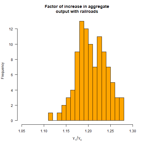
Adding the railroads increases GDP by about 20%. But: (!) Results sensitive to grid size (!) Many unrealistic assumptions
Usefulness?
This model only applies to a developing country, and is too crude to be useful for transport policy. However:
- Some model behaviour is qualitatively interesting, for example the appearance of “ghost towns”
- The idea of people being economic agents who migrate towards higher wages might be useful for forecasting regional economic development (example: current high migration from NZ to Australia)